Article Information

• Posted By : Raji Reddy A
• Posted On : May 21, 2019
• Views : 1220
• Reviews : 1
• Average User Rating :
• Recommendations : Recommended by 100% users
• Category : Predictive and Prescriptive Modeling » Machine Learning
• Description : Introduction to decision trees

Overview

• Decision Trees

  • Decision tree is a hierarchical tree structure that can be used to divide up a large collection of records into smaller sets of classes by applying a sequence of simple decision rules.
  • A decision tree model consists of a set of rules for dividing a large heterogenous population into smaller, more homogenous (mutually exclusive) classes.
  • The attributes of the classes can be any type of variables from binary, nominal, ordinal and quantitative values, while the classes must be qualitative type (categorical or binary, or ordinal).
  • In short, given a data of attributes together with its classes, a decision tree produces a sequence of rules ( or series of questions ) that can be used to recognize the class.
  • One rule is applied after another, resulting in a hierarchy of segments within segments. The hierarchy is called a tree, and each segment is called a node.
  • With each successive division, the members of the resulting sets become more and more similar to each other.
  • Hence, the algorithm used to construct decision tree is referred to as recursive partitioning.
  • The algorithm is popularly known as CART - Classification And Regression Trees.

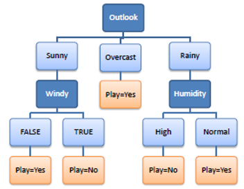
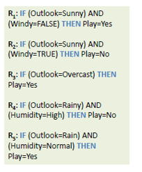
   Example:

   

  

  Consider the above scenario of a factory where

  • Expanding factor costs $1.5 million, probability of good economy is 0.4 (40%) which leads to $6 million profit and probability of bad economy is 0.6 (60%) which leads to $2 million profit.
  • Not expanding factor with $0 cost, probability of good economy is 0.4 which leads to $3M profit and probability of bad economy is 0.6 which leads to $1M profit.

  The management needs to take a decision to expand or not based on the above data,

  NetExpand  = ( 0.4 * 6 + 0.6 * 2) - 1.5 = $2.1M

  NetNo Expand  = ( 0.4 * 3 + 0.6 * 1) - 0 = $1.8M

  $2.1M > $1.8M, therefore the factory should be expanded
  

  Applications:

  • Predicting tumor cells as benign or malignant
  • Classifying credit card transactions as legitimate or fraudulent
  • Classifying buyers from non-buyers
  • Decision on whether or not to approve a loan
  • Diagnosis of various diseases based on symptoms and profile.

   Types of decision trees:

  • The target variable is usually categorical and the decision tree is used either to calculate the probability that a given record belong to each of the category or to classify the record by assigning it to the most likely class ( or category).
  • Decision tree can also be used to estimate the value of a continuous target variable. However, regression models and neural network are generally more appropriate for such estimations.

   Regression Vs. Decision Trees

   Regression Methods

  • If the relation between Y and X1, X2,....Xn is determined by linear relationship
  • When data/sample is limited
  • Extrapolation is possible when representative scenarios not present in training dataset

  Decision Trees

  • If there is a high non-linearity & complex relationship between Y and X1, X2,....Xn
  • Decision tree models are even simpler to interpret than regression!
  • When huge data is available to covering all scenarios
  • A scenario not present in training is largely misinterpreted

   Finally, accuracy of the regression methods and decision trees can be compared to decide which model to use.

   Structure of a decision tree:

    

  

   

  Types of decision tree structures:

  • Binary trees - only 2 choices in each split. Can be non-uniform (uneven) in depth
  • N-way trees or ternary trees - 3 or more choices in atleast one of its splits (3-way, 4-way etc.)

  Which node to choose for splitting?

  The best split at root (or child) nodes is defined as the one that does the best job of separating the data into groups where a single class(either 0 or 1) predominates in each group.

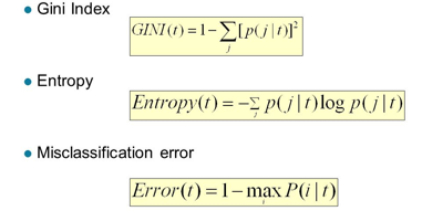
  The measure used to evaluate a potential split is purity. The best split is one that increases purity of the sub-sets by the greatest amount. There are different indicators of purity:

   

   

   

  Example of purity calculation:

   

  

   

  In the above scenario, the purity of Node N3 can be calculated as follows:

   Probability of Class = 0 & Class = 1 are equal i.e. (3/6)

  Node N3:

  Gini = 1 - ( (3/6)2 + (3/6)2 ) = 0.5

  Entropy = -(3/6) log2(3/6) - (3/6) log2(3/6) = 1

  Error = 1 - max[(3/6), (3/6)] = 0.5

  Similarly, any one of the above indicators can be calculated for Node N1, N2 and the node with highest value is chosen as the attribute to split further.

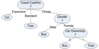
   Example ( Transportation study):

  Consider the following data which is supposed to be a part of transportation study by a government to understand travelling preferences of citizens.

  Prediction variable is mode of transportation preference: Bus, Car or Train among commuters along a major route in a city.

  The data have 4 variables.

  1. Gender is binary type
  2. Car ownership is nominal type (0 - No car, 1 - Diesel, 2 - Petrol)
  3. Travel cost/km is quantitative of ratio converted into ordinal type
  4. Income type is ordinal type

   

  
  
  
  
  

  Calculate the entropy before the split:

  P(Bus) = P(B) = 4/10 = 0.4

  P(Car) = P(C) = 3/10 = 0.3

  P(Train) = P(T) = 3/10 = 0.3

  Entropy = -0.4 log(0.4) - 0.3 log(0.3) - 0.3 log(0.3) = 1.57

  Round 1:

  Calculate the entropy of split based on gender.

  
  
  P(Female) = 5/10 = 0.5

  P(Male) = 5/10 = 0.5

  EntropyGender = 1.52 * 0.5 + 1.37 * 0.5 = 1.45

  Entropy before this split = 1.57

  Gender Entropy Gain = 1.57 - 1.45 = 0.12

   Entropy of split base on  Car Ownership:

   

   

  P(ownership = 0) = 3/10 = 0.33

  P(ownership = 1) = 5/10 = 0.5

  P(ownership = 2) = 2/10 = 0.2

  Entropyownership = 0.92*0.33 + 1.52 * 0.5 + 0*0.2 = 1.06

  Entropy before this split = 1.57

  Car Ownership Entropy Gain = 1.57 - 1.06 = 0.51

  Similaryly,

  Income Level Entropy Gain = 0.695

  Travel Cost/Km Entropy Gain = 1.210

   

   

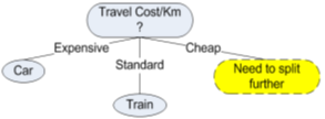
  The entropy of Travel Cost/Km is the highest. So, the decision tree should be split with Travel Cost/Km as the root node.

  After splitting, the data is as follows,

   

   

  

   

  • When the Travel Cost/Km is Expensive, Car is  the preferred mode of transportation
  • When it is Standard, Train is the preferred
  • When it is Cheap, the data should be further split as it contains both Bus and Train

   Data when Travel Cost/Km is Cheap:

   

   

  P(Bus) = P(B) = ( 4/5 ) = 0.8

  P(Train) = P(T) = ( 1/5 ) = 0.2

  P(Car) = P(C) = 0

   Entropy = -0.8 log(0.8) - 0.2 log(0.2) = 0.72

  Now repeat the above process and calculate entropy gain for each attribute Gender, Car Ownership, Income  until final decision tree is obtained.

   

  

   

   

  Decision Tree in R:

  Carseats is an inbuilt dataset used to predict sales based on other variables. Attach function can be used to load entire dataset into memory and to address variables directly instead of ‘$’ notation.
  

  attach(Carseats)
  head(Carseats)

   

   

  Convert the prediction variable Sales into binary

  High = ifelse(Sales>=8,"Yes","No")
  Carseats = data.frame(Carseats, High)

  Create training and testing data set

  set.seed(2)
  train = sample(1:nrow(Carseats),nrow(Carseats)/2)
  test = -train
  training_data = Carseats[train,]
  testing_data = Carseats[test,]
  testing_High = High[test]

  Create a Decision tree with minsplit and Minbucket parameters. minsplit is the minimum number of observations that must exist in a node in order for a split to be attempted. minbucket is the minimum number of observations in any terminal node.

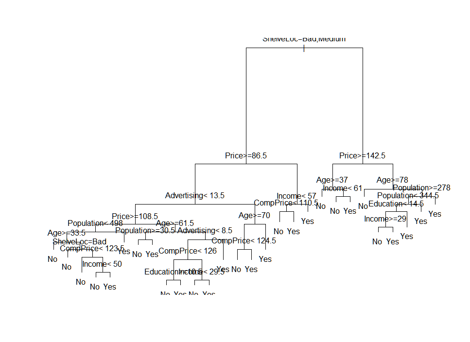
  rpart function is used to create the decision tree.

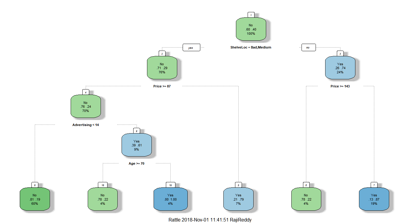
  tree1 = rpart(High ~ Income + Advertising + Population + Price + CompPrice + Age + Education + Urban + US + ShelveLoc,data=training_data,method="class",minsplit = 1, minbucket = 1)

  Plot the decision tree with inbuilt functions

  plot(tree1)
  text(tree1, pretty = 1)

   

  

  Plotting the decision tree with rattle function
  

  fancyRpartPlot(tree1)

  

   

  Predict test data using the decision tree created and calculate accuracy

  tree_pred1 = predict(tree1, testing_data, type="class")
  er1 = mean(tree_pred1 != testing_High)
  Accu1 = 1-er1
  Accu1

  Output:

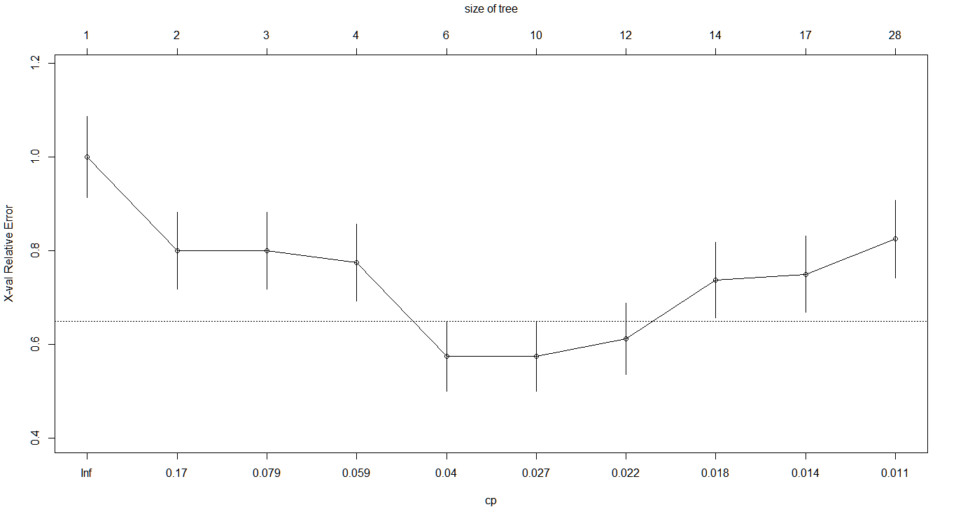
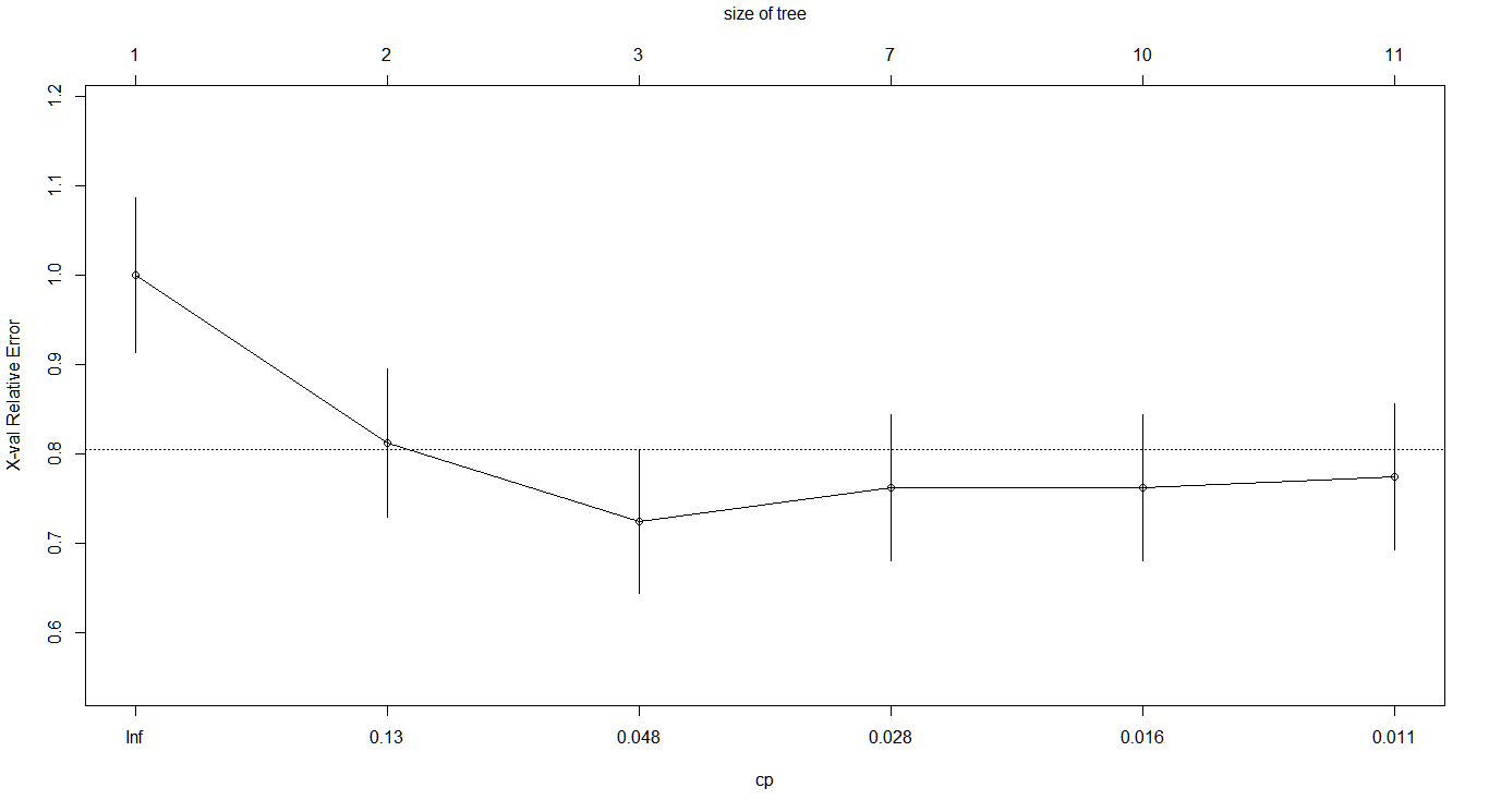
  [1] 0.775

  Complexity Parameter (cp):

  The complexity measure is a combination of the size of a tree and the ability of the

  tree to separate the classes of the target variable. Print the complexity parameter and visualized its graph.

  printcp(tree1)
  plotcp(tree1)

  Output:

   

   

  

   

  In the above table and plot, it can be observed that xerror decreases until 6th row and it increases again, this is an indication of where the optimal value of cp lies.

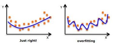
  Over-fitting and Pruning:

  Over-fitting happens when

  • Model is too complicated
  • Model works well on training data and performs very badly on test data

   Over-fitting results in decision trees that are more complex than necessary and training error no longer provides a good estimate of how well the tree will perform on previously unseen records

   

  

   

  Over-fitting can be avoided by pruning i.e. preventing  the tree from further splits.

  Pre-Pruning (Early stopping rule)

  Stop the algorithm before it becomes a fully-grown tree

  Typical stopping conditions for a node:

  • Stop if all instances belong to the same class
  • Stop if all the attributes values are the same

  More restrictive conditions:

  • Stop if number of instances is less than some user-specified threshold
  • Stop if expanding the current node does not improve impurity measures (e.g. gini or information gain)

  Post-Pruning:

  • Grow decision tree to its entirety
  • Trim the nodes of the decision tree in a bottom-up fashion
  • If generalization error improves after trimming, replace sub-tree by a leaf node

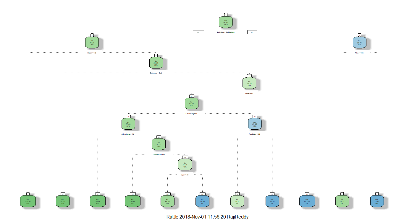
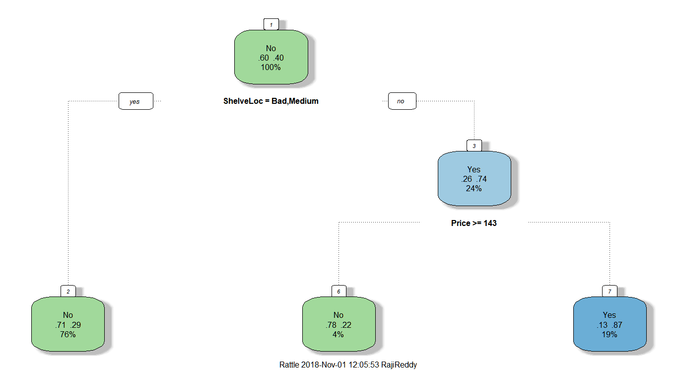
  Build a pruned tree based on complexity parameter (cp) and plot it

  ptree1 =  prune(tree1,cp= tree1$cptable[which.min(tree1$cptable[,"xerror"]),"CP"])
  fancyRpartPlot(ptree1)

  

   

   

  Predict test data using pruned decision tree and compute accuracy

  tree_predp1 = predict(ptree1, testing_data, type="class")
  erp1 = mean(tree_predp1 != testing_High) # misclassification error
  Accup1 = 1-erp1
  Accup1

  [1] 0.755

   

  Decision tree using information gain:

  rpart by default uses gini score to create leaf nodes(Terminal nodes). Create a decision tree using information gain

  tree3 = rpart(High ~ Income + Advertising + Population + Price + CompPrice +
                Age + Education + Urban + US + ShelveLoc, data=training_data,
                method="class", parms = list(split = 'information'))
  fancyRpartPlot(tree3)

   

  

   

  Accuracy:

  tree_pred3 = predict(tree3, testing_data, type="class")
  er3 = mean(tree_pred3 != testing_High) # misclassification error
  Accu3 = 1-er3
  Accu3

   

  [1] 0.74

   Prune the tree based on cp:

  printcp(tree3)
  plotcp(tree3)

   

   

  

   

  ptree3 = prune(tree3,
           cp= tree3$cptable[which.min(tree3$cptable[,"xerror"]),"CP"])
  fancyRpartPlot(ptree3)

   

  

   

   

  tree_predp3 = predict(ptree3, testing_data, type="class")
  erp3 = mean(tree_predp3 != testing_High)
  Accup3 = 1-erp3
  Accup3

   

  [1] 0.705

   

  Business Lens:

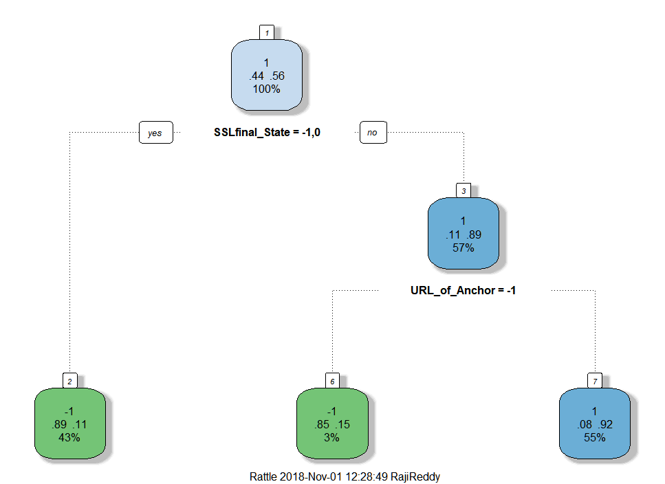
  Consider a problem where a person is assigned with identifying websites which do phishing. Phishing is an attempt to obtain sensitive information such as passwords, credit card details for malicious reasons by disguising as a trustworthy entity.

  The task is to identify and block such dangerous attempts. The data which consists of more than 8000 rows has the following features.

   

   
   

   Each column has values -1, 1, 0. -1 indicates False/negative, 1 is for True/positive, 0 is for not_sure/suspicious.

   In the Result column, 1 indicates that the website is a phishing/malicious website and -1 is for non-phishing or safe website..

   As the data in all the columns are categorical in nature, the columns should be converted to factors before creating the model.

  input = as.data.frame(lapply(originaldata, factor))

   The lapply function applies factor method on all the columns of the originaldata and gives the output in list format which is then converted to dataframe by as.data.frame().

  Divide the data into 2 groups for training and  testing.

  set.seed(123)
  train = sample(1:nrow(input),nrow(input)*.8)
  test = -train
  training_data = input[train,]
  testing_data = input[test,]
  testing_Result = Result[test]

  Create a decision tree and plot it

  tree1 = rpart(Result ~.,data=training_data,method="class")
  fancyRpartPlot(tree1)

  

   

   

  Predict test data using the decision tree computed and check accuracy

  tree_pred1 = predict(tree1, testing_data, type="class")
  er1 = mean(tree_pred1 != testing_Result)
  Accu1 = 1-er1
  Accu1

   

  [1] 0.9095534

  The accuracy of the model is 90%