Article Information
- Posted By : Raji Reddy A
- Posted On : May 22, 2019
- Views : 779
- Reviews : 1
- Average User Rating :
- Recommendations : Recommended by 100% users
- Category : Data Preparation
- Description : An explanation of factor analysis with examples
Overview
Factor Analysis is a technique of expressing observed variables in the form of potentially lower number of latent variables called factors. In a given dataset, highly correlated variables can be grouped into factors which helps in reducing the number of variables to work with, which is called as reducing the dimensionality.
When dealing with large datasets, factor analysis can be used to group several variables into few categories which focus on key components of each variable.
There are 2 important decisions to make when using factor analysis on data:
- Number of factors to choose
- Type of rotation method to choose
Mathematics Lens:
Factor analysis finds the location of the axes that fits the data better by rotating the axes. The rotation makes the factors more understandable. Rotations can be orthogonal or oblique.
Orthogonal Rotation:
Orthogonal rotation does not allow the factors to be correlated by always restricting the angle between the axes to 90 degrees. Varimax, Equimax, Quartimax are the types of Orthogonal rotation.
The Blue lines indicate the new x and y-axes after orthogonal transformation
Oblique Rotation:
Oblique rotation allows the factors to be correlated by allowing the angle between the axes to be less than 90 degrees. Direct Oblimin, Promax methods use Oblique rotation for factor analysis.
The Blue lines indicate the new x and y-axes after applying Oblique rotation
Technology Lens:
Consider the following dataset of rating given to each subject by 300 students.
Have a look at the first 10 rows.

In R, the correlation matrix can be generated by `cor()` command.
corMat = cor(my.data)
Output:

From the above table, we can infer the following:
- BIO, GEO, CHEM have better correlations with each other.
- ALG, CALC are correlated with each other.
- STAT has low correlation with other variables.
Factor Analysis with No Rotation:
n.factors = 3 fit = factanal(my.data, n.factors, rotation="none", scores="regression") fit #Check Loadings fit$loadings load = fit$loadings[,] load
Output:
Takeaways from the above output:
- Factor1 explains the majority of variance in BIO, GEO, CHEM
- Factor2 explains the majority of variance in ALG, STAT
- Factor3 does not explain anything significantly, so, it can be omitted.
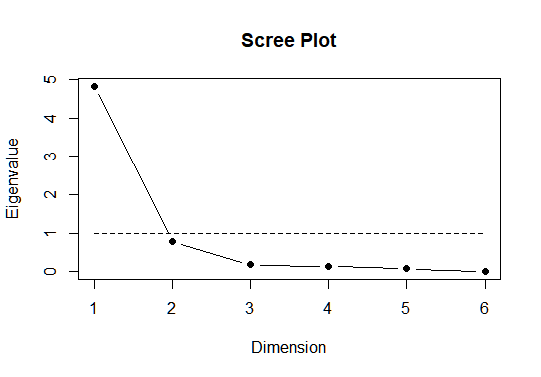
Eigenvalue is a good indicator to confirm how many factors to use. The scree plot can be used to plot the eigenvalues of the factors involved, it shows the number of factors on x-axis and eigenvalues on y-axis.
scree.plot(fit$correlation)
Generally, factors with eigenvalues >= 1 (horizontal dashed line) are good to use for the analysis. But sometimes, this rule might leave us with more than necessary number of factors or leave out the important factors whose eigenvalue is just below 1. In our example, Factor2 is slightly less than 1, both Factor1 and Factor2 can be used to explain 5 out of 6 variables.
Factor Analysis with Orthogonal Rotation - Varimax:
n.factors = 2 fit = factanal(my.data, n.factors, rotation="varimax", scores="regression") load = fit$loadings[,] load
Output:
- Factor1 explains the majority of variance in BIO, GEO, CHEM
- Factor2 explains ALG, CALC
- STAT is not explained significantly by any factor. So, it should be used as a standalone variable.
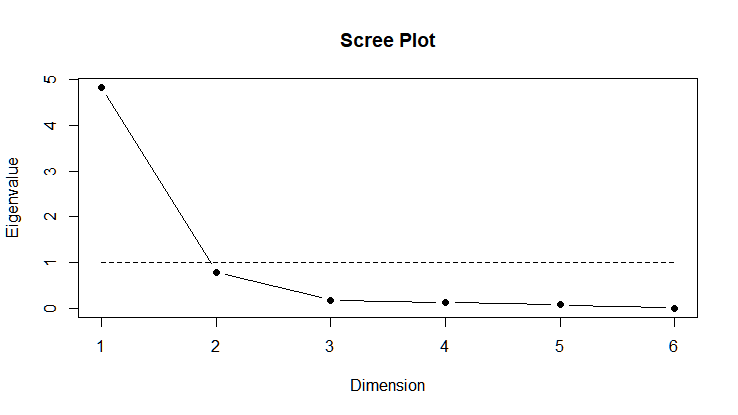
scree.plot(fit$correlation)
This scree plot similar to the one with no rotation but here Factor1 is able to explain 3 variables BIO, GEO, CHEM and Factor2 explains ALG, CALC. STAT should be considered as a standalone feature as it is not explained by any factor.
NOTE:
“None”, “Varimax” are both orthogonal rotations.
Factor Analysis with Oblique Rotation - Oblimin:
n.factors = 2 fit = factanal(my.data, n.factors, rotation="oblimin", scores="regression") load = fit$loadings[,] load
Output:

- Factor1 explains the majority of variance in BIO, GEO, CHEM
- Factor2 explains ALG and CALC
- STAT is again not explained by any factor.
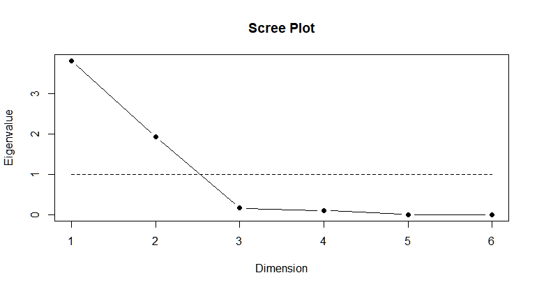
scree.plot(fit$correlation)
As in the case of varimax rotation, Factor1 and Factor2 can be used to replace 5 out of 6 features and STAT should be used as standalone feature as it is not explained by any factor.
Businesses needs to deal with many features/variables to predict a single outcome. In such cases, dimensionality reduction and the use of latent variables to explain unmeasurable traits play key role in building a better prediction model. For example, latent variables like intelligence, social anxiety, happiness cannot be measured directly but can be measured through the relationships they cause in a set of variables.
Business Lens:
Factor Analysis is widely used in psychological research and assessment scales like customer satisfaction, perceptions which cannot be measured directly. Initially, the customer/subject is provided with large set of questions which are usually answered on a numeric scale like 1-10. Then the psychological state can be indirectly measured based on the responses provided by the subject.
Investing relies on data analysis to take vital decisions. Factor analysis is used in stock market strategies where it is important to find out why a stock is performing better or worse. Other areas like human resource staffing, education and insurance companies also rely on factor analysis for effective policies and decision making.
Let’s look at a business problem of a Tooth paste brand which wants to get an insight on customers’ behavioral pattern to price and promote their product accordingly.
The company does a disguised survey where the customers can rate the relative importance of the following attributes on a scale 1-Least Important to 7-Most Important.
- Cavity prevention
- Improve shine of the teeth
- Improve gum strength
- Fresh breath
- Price
- Instant results
Here is the sample data from the survey:

The correlations between the above features are as follows:
corMat = cor(myData) corMat
A negative correlation between 2 variables indicates that when one variable increases, the other decreases and vice versa. Generally, anything above 0.7 can be considered a good correlation. As we can see in the above table, there is a correlation between the variables, hence, factor analysis can be performed on the data.
n.factors = 2 fit = factanal(myData, n.factors, rotation="oblimin", scores="regression") loadings = fit$loadings[,] loadings
Output:

- Factor1 explains PreCavity, StrongGum, Price
- Factor2 explains ShinyTeeth, FreshBreath, Instanteffect
scree.plot(fit$correlation)
What can we infer from the survey?From the above analysis, the participants in the survey can be categorised into 2 groups, one that prioritizes health of their teeth and the other group that prefers visual appearance of their teeth. Based on this, the company can take a decision to promote their toothpaste brand to appeal to the either of the group or they can manufacture separate products for each group of people. Another interesting observation is that price is highly and inversely correlated with PreCavity and StrongGum which can be an indication that people prefering health of their teeth are not much bothered about the price of the product. Thus, the company can also plan the pricing of their product from this analysis.