Multiple Linear Regression
Multiple Linear Regression is basically indicating that we will be having many features Such as f1, f2, f3, f4, and our output feature f5. If we take the same example as above we discussed, suppose:
f1 is the size of the house.
f2 is bad rooms in the house.
f3 is the locality of the house.
f4 is the condition of the house and,
f5 is our output feature which is the price of the house.
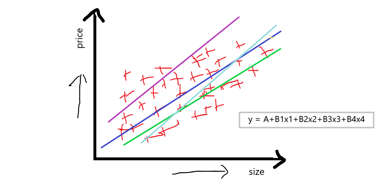
Now, you can see that multiple independent features also make a huge impact on the price of the house, price can vary from feature to feature. When we are discussing multiple linear regression then the equation of simple linear regression y=A+Bx is converted to something like:
equation: y = A+B1x1+B2x2+B3x3+B4x4
“If we have one dependent feature and multiple independent features then basically call it a multiple linear regression.”
Now, our aim to using the multiple linear regression is that we have to compute A which is an intercept, and B1 B2 B3 B4 which are the slops or coefficient concerning this independent feature, that basically indicates that if we increase the value of x1 by 1 unit then B1 says that how much value it will affect int he price of the house, and this was similar concerning others B2 B3 B4
So, this is a small theoretical description of multiple linear regression now we will use the scikit learn linear regression library to solve the multiple linear regression problem.
Dataset
Now, we apply multiple linear regression on the 50_startups dataset, you can click here to download the dataset.
Reading dataset
Most of the dataset are in CSV file, for reading this file we use pandas library:
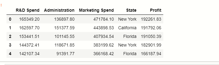
df = pd.read_csv('50_Startups.csv')
df
Here you can see that there are 5 columns in the dataset where the state stores the categorical data points, and the rest are numerical features.
Now, we have to classify independent and dependent features:
Independent and Dependent variables
There are total 5 features in the dataset, in which basically profit is our dependent feature, and the rest of them are our independent features:
#separate the other attributes from the predicting attribute
x = df.drop('Profit',axis=1)
#separte the predicting attribute into Y for model training
y = ['profit']
Handling categorical variables
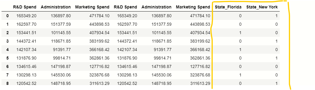
In our dataset, there is one categorical column State, we have to handle this categorical values present inside this column for that we will use pandas get_dummies() function:
# handle categorical variable
states=pd.get_dummies(x,drop_first=True)
# dropping extra column
x= x.drop(‘State’,axis=1)
# concatation of independent variables and new cateorical variable.
x=pd.concat([x,states],axis=1)
x
Splitting Data
Now, we have to split the data into training and testing parts for that we use the scikit-learn train_test_split() function.
# importing train_test_split from sklearn
from sklearn.model_selection import train_test_split
# splitting the data
x_train, x_test, y_train, y_test = train_test_split(x, y, test_size = 0.2, random_state = 42)
Applying model
Now, we apply the linear regression model to our training data, first of all, we have to import linear regression from the scikit-learn library, there is no other library to implement multiple linear regression we do it with linear regression only.
# importing module
from sklearn.linear_model import LinearRegression
# creating an object of LinearRegression class
LR = LinearRegression()
# fitting the training data
LR.fit(x_train,y_train)
finally, if we execute this then our model will be ready, now we have x_test data we use this data for the prediction of profit.
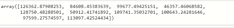
y_prediction =  LR.predict(x_test)
y_prediction
Now, we have to compare the y_prediction values with the original values because we have to calculate the accuracy of our model, which was implemented by a concept called r2_score. let’s discuss briefly on r2_score:
r2_score:-
It is a function inside sklearn. metrics module, where the value of r2_score varies between 0 and 100 percent, we can say that it is closely related to MSE.
r2 is basically calculated by the formula given below:
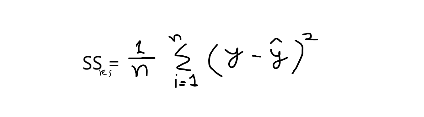
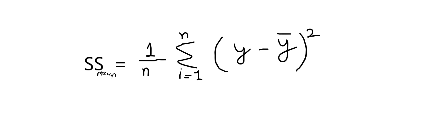
formula: r2 = 1 – (SSres /SSmean )
now, when I say SSres it means, it is the sum of residuals and SSmean refers to the sum of means.
where,
y = original values
y^ = predicted values. and,
If we take calculation from this equation, then we have to know that the value of the sum of means is always greater than the sum of residuals. If this condition satisfies then our model is good for predictions. Its values range between 0.0 to 1.
”The proportion of the variance in the dependent variable that is predictable from the independent variable(s).”
The best possible score is 1.0 and it can be negative because the model can be arbitrarily worse. A constant model that always predicts the expected value of y, disregarding the input features, would get an R2 score of 0.0.
# importing r2_score module
from sklearn.metrics import r2_score
from sklearn.metrics import mean_squared_error
# predicting the accuracy score
score=r2_score(y_test,y_prediction)
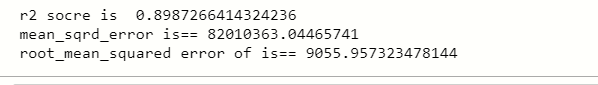
print(‘r2 socre is ‘,score)
print(‘mean_sqrd_error is==’,mean_squared_error(y_test,y_prediction))
print(‘root_mean_squared error of is==’,np.sqrt(mean_squared_error(y_test,y_prediction)))
You can see that the accuracy score is greater than 0.8 it means we can use this model to solve multiple linear regression, and also mean squared error rate is also low.