SELECT primary_type,block, COUNT(*) as count
FROM `bigquery-public-data.chicago_crime.crime`
HAVING COUNT(*) = (SELECT MAX(count)
FROM (SELECT primary_type, COUNT(*) as count FROM `bigquery-public-data.chicago_crime.crime` GROUP BY primary_type, block) `bigquery-public-data.chicago_crime.crime`)#standardSQL
SELECT
block,
ARRAY_AGG(STRUCT(primary_type, cnt) ORDER BY cnt DESC LIMIT 1)[OFFSET(0)].*
FROM (
SELECT
block,
primary_type,
COUNT(*) cnt
FROM `bigquery-public-data.chicago_crime.crime`
GROUP BY block, primary_type
)
GROUP BY blockThis should give you the top frequent crime by block
Inner query count calculates the frequency of crime, window partitioning function calculates the rank based on descending order of crime frequency partitioned by block. outer query where clause rank =1 return only the top frequent crime. you can change outer query where clause to get top 5 frequent crime by making it rank <=5
select * from
      (SELECT block, primary_type, count(primary_type) as crime_frquency,
            ROW_NUMBER() OVER (PARTITION BY block ORDER BY count(primary_type) DESC) AS rank
       FROM  `bigquery-public-data.chicago_crime.crime`
       group by block, primary_type)
where rank = 1WHERE _PARTITIONTIME
BETWEEN TIMESTAMP("20160101")
AND TIMESTAMP("20160131")Let’s look at the pricing for BigQuery, then explore each billing subcategory to offer tips to reduce your BigQuery spending. For any location, the BigQuery pricing is broken down like this:
Storage
Active storage
Long-term storage
Streaming inserts
Query processing
On-demand
Flat-rate
Before we dive deeper into each of those sections, here are the BigQuery operations that are free of charge in any location:
Batch loading data into BigQuery
Automatic re-clustering (which requires no setup and maintenance)
Exporting data operation
Deleting table, views, partitions, functions and datasets
Queries that result in error
Storage for first 10 GB of data per month
Query data processed for first 1 TB of data per month (advantageous to users on on-demand pricing)
Once data is loaded into BigQuery, charges are based on the amount of data stored in your tables per second. Here are a few tips to optimize your BigQuery storage costs.
1. Keep your data only as long as you need it.
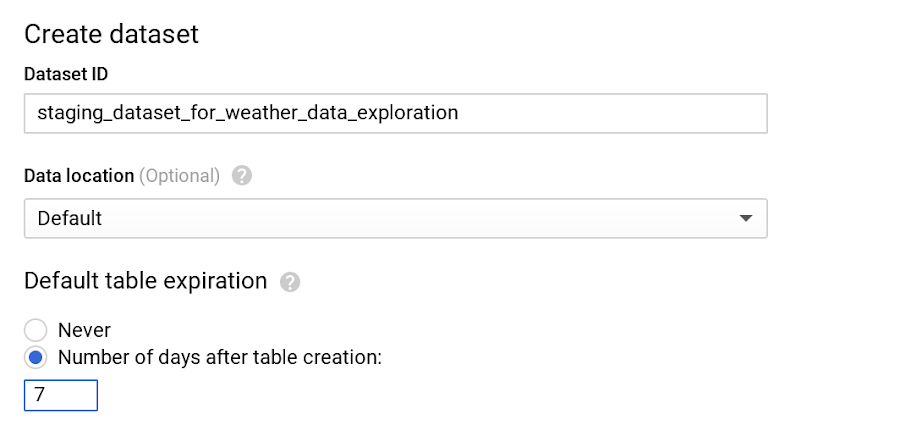
By default, data stored in BigQuery’s Capacitor columnar data format is already encrypted and compressed. Configure default table expiration on your dataset for temporary staging data that you don’t need to preserve.
For instance, in this example, we only need to query the staging weather dataset until the downstream job cleans the data and pushes it to a production dataset. Here, we can set seven days for the default table expiration.
Note that if you’re updating the default table expiration for a dataset, it will only apply to the new tables created. Use DDL statement to alter your existing tables.
BigQuery also offers the flexibility to provide different table expiration dates within the same dataset. So this table called new_york in the same dataset needs data retained for longer.
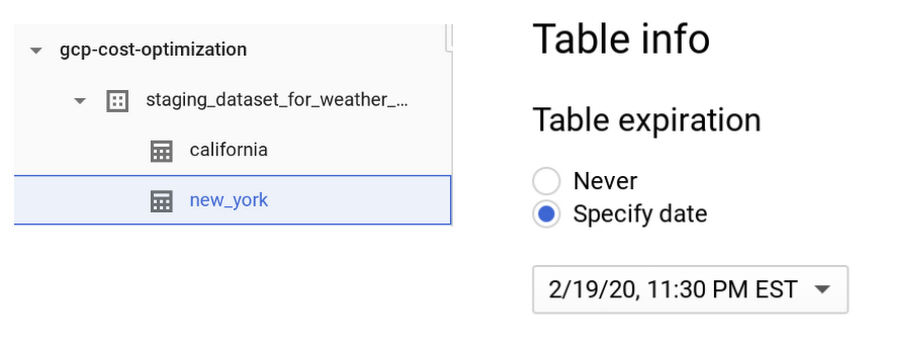
As shown in the image above, new_york will retain its data for six months, and because we haven’t specified table expiration for california, its expiration will default to seven days.
Pro tip: Similar to dataset-level and table-level, you can also set up expiration at the partition level. Check out our public documentation for default behaviors.
2. Be wary of how you edit your data.
If your table or partition of a table has not been edited for 90 days, the price of the data stored in the table automatically drops by about 50%. There is no degradation of performance, durability, availability or any other functionality when a table or partition is considered for long-term storage.
To get the most out of long-term storage, be mindful of any actions that edit your table data, such as streaming, copying, or loading data, including any DML or DDL actions. This will bring your data back to active storage and reset the 90-day timer. To avoid this, you can consider loading the new batch of data to a new table or a partition of a table if it makes sense for your use case.
Pro tip: Querying the table data along with few other actions do not reset the 90-day timer and the pricing continues to be considered as long-term storage.
In most cases, keeping the data in BigQuery is advantageous unless you are certain that the data in the table will be accessed at most once a year, like storing archives for legal or regulatory reasons. In that case, explore the option of exporting the table data into the Coldline class of a Cloud Storage bucket for even better pricing than BigQuery’s long-term storage.
3. Avoid duplicate copies of data.
BigQuery uses a federated data access model that allows you to query data directly from external data sources like Cloud Bigtable, Cloud Storage, Google Drive and Cloud SQL (now in beta!). This is useful for avoiding duplicate copies of data, thus reducing storage costs. It’s also helpful for reading data in one pass from an external source or accessing a small amount of frequently changed data that doesn’t need to be loaded in BigQuery every time it is changed.
Pro tip: Choose this technique for the use cases where it makes the most sense. Typically, queries that run on external sources don’t perform as well compared to queries executed on same data stored on BigQuery, since data stored on BigQuery is in a columnar format that yields much better performance.
4. See whether you’re using the streaming insert to load your data.
Check your last month’s BigQuery bill and see if you are charged for streaming inserts. If you are, ask yourself: “Do I need data to be immediately available (in a few seconds instead of hours) in BigQuery?” or “Am I using this data for any real-time use case once the data is available in BigQuery?” If either answer is no, then we recommend you to switch to batch loading data, as it is completely free.
Pro tip: Use streaming inserts only if the data in BigQuery is consumed immediately by downstream consumers.
5. Understand BigQuery’s backup and DR processes.
BigQuery maintains a seven-day history of changes to your table, which allows you to query a point-in-time snapshot of your data. This means you can revert back the data without restoring from recovery backups. If the table is deleted, its history is flushed after two days.
To find the number of rows from a snapshot of a table one hour ago, use the following query:
Select COUNT(*) FROM [Project_ID:Dataset.Table@-3600000]
Find more examples in the documentation.
Pro tip: For business-critical data, please follow the Disaster Recovery Scenarios for Data guide for a data backup, especially if you are using BigQuery in a regional location.
You’ll likely query your BigQuery data for analytics and to satisfy business use cases like predictive analysis, real-time inventory management, or just as a single source of truth for your company’s financial data.
On-demand pricing is what most users and businesses choose when starting with BigQuery. You are charged for the number of bytes processed, regardless of the data housed in BigQuery or external data sources involved. There are some ways you can reduce the number of bytes processed. Let's go through the best practices to reduce the cost of running your queries, such as SQL commands, jobs, user-defined functions, and more.
1. Only query the data you need. (We mean it!)
BigQuery can provide incredible performance because it stores data as a columnar data structure. This means SELECT * is the most expensive way to query data. This is because it will perform a full query scan across every column present in the table(s), including the ones you might not need. (We know the guilty feeling that comes with adding up the number of times you've used SELECT * in the last month.)
Let’s look at an example of how much data a query will process. Here we’re querying one of the public weather datasets available in BigQuery:

As you can see, by selecting the necessary columns, we can reduce the bytes processed by about eight-fold, which is a quick way to optimize for cost. Also note that applying the LIMIT clause to your query doesn’t have an effect on cost.
Pro tip: If you do need to explore the data and understand its semantics, you can always use the no-charge data preview option.
Also remember you are charged for bytes processed in the first stage of query execution. Avoid creating a complex multistage query just to optimize for bytes processed in the intermediate stages, since there are no cost implications anyway (though you may achieve performance gains).
Pro tip: Filter your query as early and as often as you can to reduce cost and improve performance in BigQuery.
2. Set up controls for accidental human errors.
The above query was on the magnitude of GB, a mishap that can cost you a few cents, which is acceptable for most businesses. However, when you have dataset tables that are in the magnitude of TBs or PBs and are accessed by multiple individuals, unknowingly querying all columns could result in a substantial query cost.
In this case, use the maximum bytes billed setting to limit query cost. Going above the limit will cause the query to fail without incurring the cost of the query, as shown below.
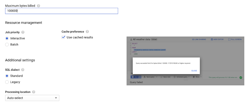
A customer once asked why custom control is so important. To put things into perspective, we used this example. Let’s say you have 10 TB of data in a U.S. (multi-regional) location, for which you are charged about $200 per month for storage. If 10 users sweep all the data using [SELECT * .. ] 10 times a month, your BigQuery bill is now about $5,000, because you are sweeping 1 PB of data per month. Applying thoughtful limits can help you prevent these types of accidental queries. Note that cancelling a running query may incur up to the full cost of the query as if it was allowed to complete.
Pro Tip: Along with enabling cost control on a query level, you can apply similar logic to the user level and project level as well.
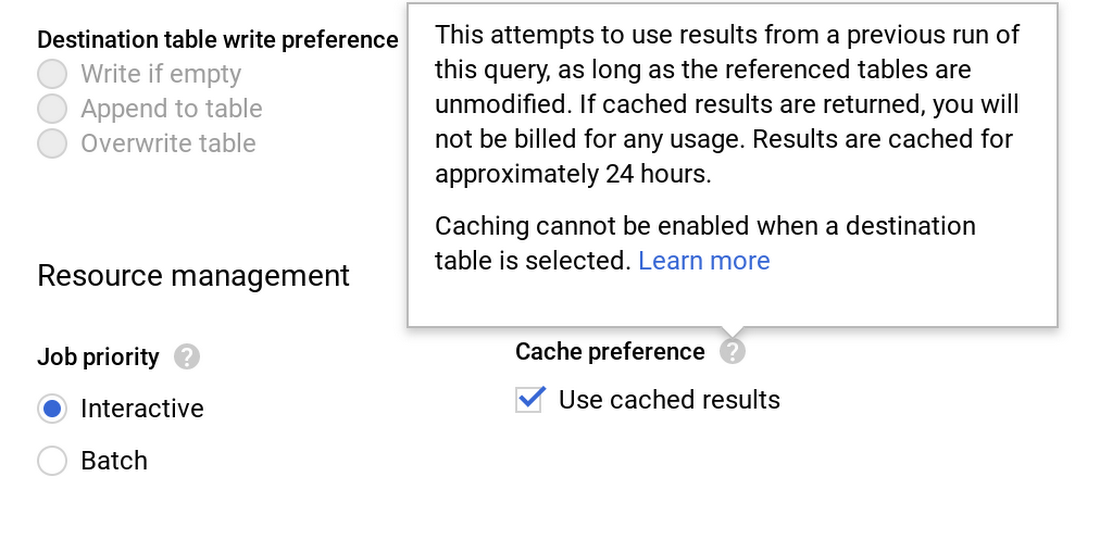
3. Use caching intelligently.
With few exceptions, caching can actually boost your query performance, and you won’t be charged for the results retrieved from the cached tables. By default, cache preference is turned on. Check them in your GCP console by clicking More -> Query settings on your query editor, as shown here.
Also, keep in mind that caching is per user, per project.
Let’s take a real-world example, where you have a Data Studio dashboard backed by BigQuery and accessed by hundreds or even thousands of users. This will show right away that there is a need for intelligently caching your queries across multiple users.
Pro tip: To significantly increase the cache hit across multiple users, use a single service account to query BigQuery, or use community connectors, as shown in this Next ‘19 demo.
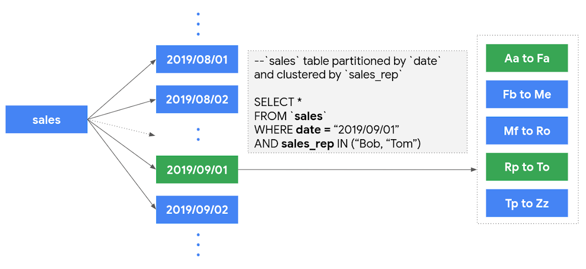
4. Partition your tables.
Partitioning your tables, whenever possible, can help reduce the cost of processing queries as well as improve performance. Today, you can partition a table based on ingestion time, date, or any timestamp column. Let’s say you partition a sales table that contains data for the last 12 months. This results in smaller partitions containing data for each day, as shown below.
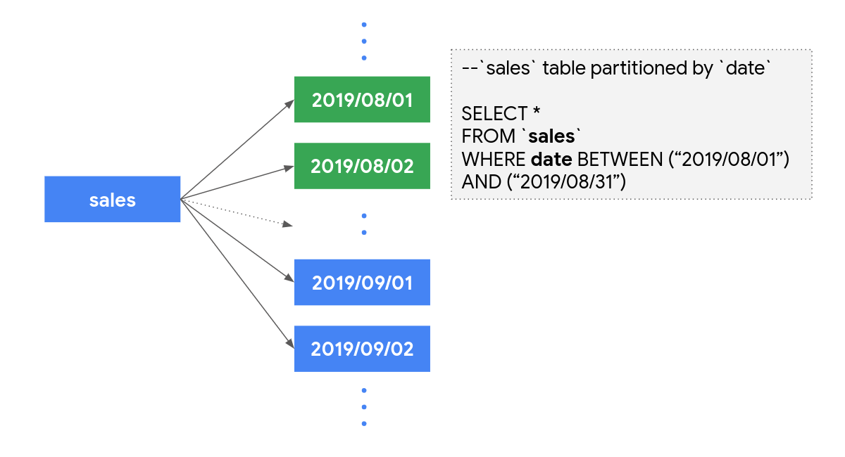
Now, when you query to analyze sales data for the month of August, you only pay for data processed in those 31 partitions, not the entire table.
One more benefit is that each partition is separately considered for long-term storage, as discussed earlier. Considering our above example, sales data is often loaded and modified for the last few months. So all the partitions that are not modified in the last 90 days are already saving you some storage costs. To really get the benefits of querying a partitioned table, you should filter the table using a partition column.
Pro tip: While creating or updating partitioned table, you can enable “Require partition filter” which will force users to include a WHERE clause that specifies the partition column, or else the query will result in error.
5. Further reduce sweeping your data using clustering.
After partitioning, you can now cluster your table, which organizes your data based on the content for up to four columns. BigQuery then sorts the data based on the order of columns specified and organizes them into a block. When you use query filters using these columns, BigQuery intelligently only scans the relevant blocks using a process referred to as block pruning.
For example, below, sales leadership needs a dashboard that displays relevant metrics for specific sales representatives. Enabling clustering order on sales_rep column is a good strategy, as it is going to be used often as a filter. As shown below, you can see that BigQuery only scans one partition (2019/09/01) and the two blocks where sales representatives Bob and Tom can be found. The rest of the blocks in that partition are pruned. This reduces the number of bytes processed and thus the associated querying cost.