Business Statistics is the science of decision making by analyzing and interpreting data using several statistical methods.
Probability Distributions
Probability is the long run average of a random event occurring. Probability distribution is a rule that identifies possible outcome of a random variable and assigns a probability to each. There are 2 types of probability distributions - Discrete and Continuous.
Discrete Distribution has a finite number of outcome values, e.g. face value of a card, number of bad cheques received by a bank, number of absent employees.
Continuous Distribution has all possible outcomes in some range, e.g. sales per month, height of students of a class. These are nicer to deal with and are good approximations when there are a large number of possible values.
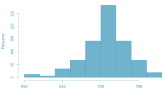
Histogram
A histogram represents the frequency distribution, i.e. how many observations take the value within a certain interval - e.g. GMAT scores
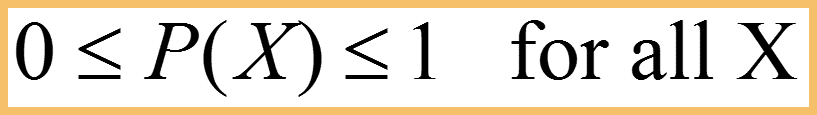
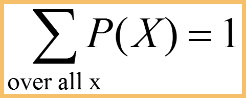
Requirements for a Discrete Probability Function
For example, the hourly sales of google pixel on flipkart can be shown as below,
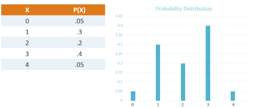
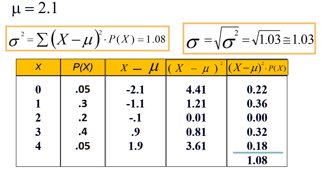
Expected Value or Mean of a random variable is the weighted average of its values.
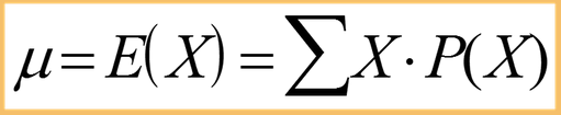
By the above formula, the mean number of google pixel phones sold per hour in the above graphic can be calculated as, (0*0.05 + 1*0.3 + 2*0.2 + 3*0.4 + 4*0.05) = 2.1
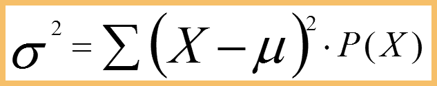
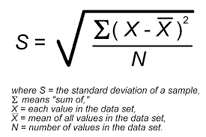
Variance (σ2) is the weighted average of the squared deviations from the mean. Variance measures how far a dataset is spread out. The technical definition is “The average of the squared differences from the mean”, but all it really does is give a general idea of the spread of the data. A value of zero means that there is no variability. The probabilities serve as weights and units are square of the units of the variable.
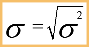
Standard Deviation (σ) : The Square root of variance is the standard deviation. While variation gives rough idea of spread of a dataset, the standard deviation is more concrete, giving exact distances from the mean. It has same units as the variable.
Uniform Distribution is characterized by flat distribution. Imagine rolling a fair die, the outcomes 1 to 6 are equally likely. It can be defined for any number of outcomes n or even as a continuous distribution.

Bernoulli Distribution has two lines of equal height, representing the two equally probable outcomes of 0 and 1 at either end. Eg: Two discrete outcomes - tails or heads.

Binomial Distribution is the sum of outcome of things that follow a bernoulli distribution. If the need is for counting the number of successes in things that act like a coin flip, where each flip is independent and has the same probability of success. Binomial distribution is denoted by the notation b(k;n,p);
b(k;n,p) = C(n,k) pk qn-k, where C(n,k) is known as the binomial coefficient.

Hypergeometric Distribution is similar count like binomial but without the replacement of events. It is definitely close to binomial distribution but not the same, because the probability of success changes as the trial is measured without replacement.

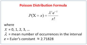
Poisson Distribution is also the distribution of a count - the count of times something happened. It is parameterized not by a probability p and number of trials n but by an average rate λ, which in this analogy is simply the constant value of np. The poisson distribution is what one can use when trying to count events over a time given the continuous rate of events occuring.
When things like packets arrive at routers, or customers arrive at a store, or things wait in some kind of queue, think poisson.

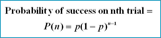
Geometric Distribution is the probability of success in Nth trial

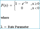
Exponential Distribution - Given events whose count per time follows a poisson distribution, then the time between events follows an exponential distribution with the same rate parameter λ. The exponential distribution should come to mind when thinking of “time until event”, maybe “time until failure”.

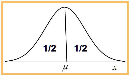
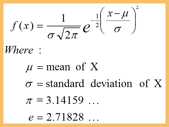
Normal Distribution
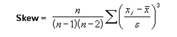
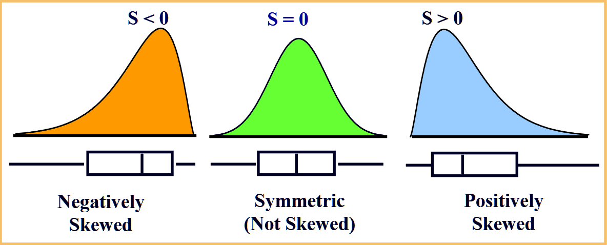
Coefficient of Skewness
Skewness is the measure of asymmetry in one variable of a data.
Kurtosis
A positive kurtosis value means that there is too little data in the tails. A negative value means there is too much data in the tails. The heaviness or lightness in the tails means that the data looks less peaked (or more peaked).
Kurtosis is measured against the standard normal distribution. The standard normal distribution has a kurtosis of 3, so if the values are closer to that then the graph is nearly normal. These nearly normal distributions are called mesokurtic.
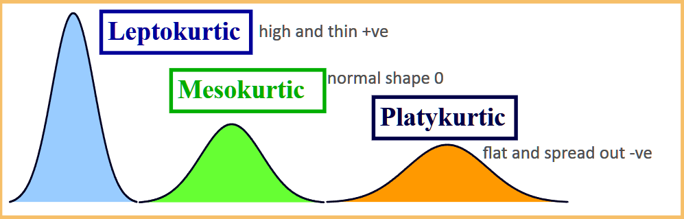
Excess kurtosis is just kurt-3. For example, the excess for the normal distribution is 3-3=0.
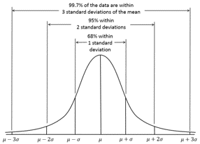
Normal distribution with a width of 1, 2 and 3 standard deviations
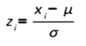
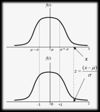
Z-Scores, Standard Normal Distribution
For every value of (x) of the random variable X, we can calculate its Z-score.
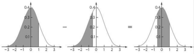
If X~N(μ,σ2), then Z-scores have a normal distribution with μ=0, σ=1 i.e. Z~N(0,1). This is called Standard Normal Distribution. Z-table only gives less than probabilities.
Z-Tables
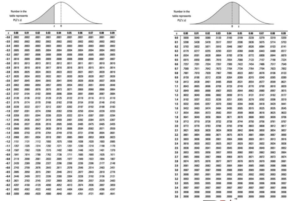
Probability Calculation for Normal Distribution
Suppose GMAT scores can be reasonably modelled using a normal distribution with μ = 711 and σ = 29, P(X<=680) can be calculated as follows
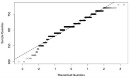
Normal-Quantile (Q-Q) plot
The Central Limiting Theorem states that the distribution of the sample mean
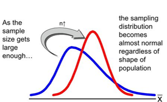
Applications of Central Limit Theorem (CLT)