Logistic regression is intended for the modelling of dichotomous categorical outcomes (e.g., dead vs. alive, cancer vs. none, buy vs. does not buy). Logistic and linear regression are both based on many of the same assumptions and theory.

As an alternative to modelling the value of the outcome, logistic regression focuses instead upon the relative probability (odds) of obtaining a given result category.

Where p represents the probability of an event (e.g., buy), b0 is the y-intercept, and x1 to xk  represent the independent variables included in the model. As with the linear model, each independent variable’s association with the outcome (log odds) is indicated by the coefficients b1 to bk.

An error term is included to account for differences between the observed outcome values and those predicted by the model. In effect, we are trying to model the probability that an event is a result of a linear combination of variables as indicated in the equation above.

Given the similarities with linear regression, the above model is also called Linear Probability Model.

Why not Linear regression?

Since E(Y | X) is a probability, it has to lie between 0 and 1. Not all predicted values lie between 0 and 1.

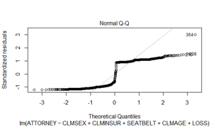
Normality can never be achieved for errors since each error takes only 2 values from QQ plot.

                                                                 

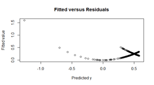
Also a quadratic trend can be observed from residuals

                                                                     

Sigmoid shape:

Consider data on house ownership. After particular level of income, the probability of a family owning a house becomes near 1. At very low levels of income, the probability of a family owning a house becomes near 0.

                                                                                         

Linearizing transformation:

Pi = E(Yi|X) =1/( 1 + e^-(β0+β1X1+β2X2+......+βiXi)  )

• Take ratio: Pi/(1-Pi) = ezi


• Then take logarithm on both sides

Li = ln(Pi/(1-Pi)) = Zi = β0+β1X1+β2X2+......+βiXi

This is called the Logit model/ Logistic Regression

• (Pi/(1-Pi)) is simply the ratio of the probability that a person buys of the house to the probability that he doesn’t. This ratio is called the odds ratio. Eg: Odds ratio = 2 means that the odds are 2 to 1 in favour of buying the house.


• If L>0, it means that as the value of the regressor increases, the odds that the regressand equals one (person buying the house) increases.


• Note that when the log odds are negative, the odds will be < 1.

Logistic Regression in R:

Consider a challenge where an insurance company wants to predict whether an insurance claimant will hire an attorney to represent him. The following variables are available in the dataset.

CASENUM - Case number to identify the claim

ATTORNEY - Whether the claimant is represented by an attorney (=0 if yes and =1 if no)

CLMSEX - Claimant's gender (=0 if male and =1 if female)

CLMINSUR - Whether or not the driver of the claimant's vehicle was insured (=0 if yes, =1 if no)

SEATBELT - Whether or not the claimant was wearing a seatbelt/child restraint (=0 if no, =1 if yes)

CLMAGE - Claimant's age

LOSS - The claimant's total economic loss (in thousands)​

• The feature CASENUM is just for identification and does not have any significance to use in the analysis.


• The features CLMSEX, CLMINSUR, SEATBELT represent yes or no values and does not have numeric significance. So, it is recommended to use them as factors.

Linear model:

Let us first use linear model to see why it is not useful in these kind of analysis.

fit = lm(ATTORNEY ~ factor(CLMSEX) + factor(CLMINSUR) + factor(SEATBELT) + CLMAGE + LOSS,data=claimants)

plot(fit)​

A quadratic trend can be observed from residuals which is indicates a inefficient prediction model

As each error ranges from -1 to 1, normality cannot be acheived with the linear model.

The model is efficient if the residuals in Scale-Location plot are distributed randomly but a pattern can be observed in the distribution of residuals.

Logistic model:

Logit = glm(ATTORNEY ~ factor(CLMSEX) + factor(CLMINSUR) + factor(SEATBELT) + CLMAGE + LOSS,family= "binomial",data=claimants)

summary(logit)​

Output:

Null deviance: 1516.1  on 1095  degrees of freedom

Residual deviance: 1287.8  on 1090  degrees of freedom

AIC: 1299.8

Null Deviance and Residual Deviance:

Null Deviance indicates the response predicted by a model with nothing but an intercept. Lower the value, better the model. Residual deviance indicates the response predicted by a model on adding independent variables. Lower the value, better the model.

AIC (Akaike Information Criteria):

The analogous metric of adjusted R² in logistic regression is AIC. AIC is the measure of fit which penalizes model for the number of model coefficients. Therefore, we always prefer model with minimum AIC value.

Confusion Matrix:

It is a tabular representation of Actual vs Predicted values. This helps to find the accuracy of the model and avoid overfitting.

prob = predict(logit,claimants,type = 'response')

confusion = table(prob>0.5,claimants$ATTORNEY)

rownames(confusion) = c("0", "1")

confusion​

Output:

The above table can be interpreted as:

True Negatives  (Predicted 0 & Actual 0): 380

False Positives   (Predicted 1 & Actual 0): 125

False Negatives (Predicted 0 & Actual 1): 198

Accuracy, sensitivity, specificity:

Accuracy = sum(diag(confusion))/sum(confusion)

Accuracy​

[1] 0.705292​

It is called as Receiver Operating Characteristic Curve. The Area Under Curve (AUC) of the ROC provides an overall measure of fit of the model.

1. It shows the tradeoff between sensitivity and specificity (any increase in sensitivity will be accompanied by a decrease in specificity).


2. The closer the curve follows the left-hand border and then the top border of the ROC space, the more accurate the test.


3. The closer the curve comes to the 45-degree diagonal of the ROC space, the less accurate the test.

predictTest = data.frame("Probability"=predict(logit,claimants, type = 'response'))

RCRTest = prediction(predictTest$Probability,claimants$ATTORNEY)

ROCRTestPerf = performance(RCRTest,"tpr","fpr")

plot(ROCRTestPerf,main="ROC Curve")

auc = paste(c("AUC ="),round(as.numeric(performance(RCRTest,"auc")@y.values), digits=2),sep="")

legend("topleft",auc, bty="n")​

It is called as pseudo R2. When analyzing data with a logistic regression, an equivalent statistic to R-Squared does not exist. However, to evaluate the goodness-of-fit of logistic models, several R-Squareds have been developed.

Rsq = pR2(logit)[4]

Rsq​

Output:

McFadden

0.3064751​

Business Lens:

Consider a problem where a person is assigned with identifying websites which do phishing. Phishing is an attempt to obtain sensitive information such as passwords, credit card details for malicious reasons by disguising as a trustworthy entity.

The task is to identify and block such dangerous attempts. The data which consists of more than 8000 rows has the following features.

In the Result column, 1 indicates that the website is a phishing/malicious website and -1 is for non-phishing or safe website..

As the data in all the columns are categorical in nature, the columns should be converted to factors before creating the model.

input = as.data.frame(lapply(originaldata, factor))​

The lapply function applies factor method on all the columns of the originaldata and gives the output in list format which is then converted to dataframe by as.data.frame().

Divide the data into 2 groups for training and  testing.

set.seed(123)

train = sample(1:nrow(input),nrow(input)*.8)

test = -train

training_data = input[train,]

testing_data = input[test,]

testing_Result = Result[test]​

Create a logistic regression model with the training data.

logit = glm(Result ~.,family= "binomial",data=training_data)​

Predict on the testing data using the above model and check the confusion matrix by considering the probabilities > 0.5 as a phishing website.

prob = predict(logit,testing_data)

confusion = table(prob>0.5,testing_data$Result)

rownames(confusion) = c("0", "1")

confusion​

Output:

Calculate the accuracy of the model:

AccuracyLg = sum(diag(confusion))/sum(confusion)

AccuracyLg​

[1] 0.9355568​

The accuracy of the model is 93%.