


Last Updated on August 19, 2020
Machine learning is a field of study and is concerned with algorithms that learn from examples.
Classification is a task that requires the use of machine learning algorithms that learn how to assign a class label to examples from the problem domain. An easy to understand example is classifying emails as “spam” or “not spam.”
There are many different types of classification tasks that you may encounter in machine learning and specialized approaches to modeling that may be used for each.
In this tutorial, you will discover different types of classification predictive modeling in machine learning.
After completing this tutorial, you will know:
- Classification predictive modeling involves assigning a class label to input examples.
- Binary classification refers to predicting one of two classes and multi-class classification involves predicting one of more than two classes.
- Multi-label classification involves predicting one or more classes for each example and imbalanced classification refers to classification tasks where the distribution of examples across the classes is not equal.
Kick-start your project with my new book Machine Learning Mastery With Python, including step-by-step tutorials and the Python source code files for all examples.
Let’s get started.
 https://machinelearningmastery.com/wp-content/uploads/2020/04/Types-of-Classification-in-Machine-Learning-300x170.jpg 300w, https://machinelearningmastery.com/wp-content/uploads/2020/04/Types-of-Classification-in-Machine-Learning-768x434.jpg 768w" alt="Types of Classification in Machine Learning" width="800" height="452">
Types of Classification in Machine Learning
Photo by Rachael, some rights reserved.
Tutorial Overview
This tutorial is divided into five parts; they are:
- Classification Predictive Modeling
- Binary Classification
- Multi-Class Classification
- Multi-Label Classification
- Imbalanced Classification
Classification Predictive Modeling
In machine learning, classification refers to a predictive modeling problem where a class label is predicted for a given example of input data.
Examples of classification problems include:
- Given an example, classify if it is spam or not.
- Given a handwritten character, classify it as one of the known characters.
- Given recent user behavior, classify as churn or not.
From a modeling perspective, classification requires a training dataset with many examples of inputs and outputs from which to learn.
A model will use the training dataset and will calculate how to best map examples of input data to specific class labels. As such, the training dataset must be sufficiently representative of the problem and have many examples of each class label.
Class labels are often string values, e.g. “spam,” “not spam,” and must be mapped to numeric values before being provided to an algorithm for modeling. This is often referred to as label encoding, where a unique integer is assigned to each class label, e.g. “spam” = 0, “no spam” = 1.
There are many different types of classification algorithms for modeling classification predictive modeling problems.
There is no good theory on how to map algorithms onto problem types; instead, it is generally recommended that a practitioner use controlled experiments and discover which algorithm and algorithm configuration results in the best performance for a given classification task.
Classification predictive modeling algorithms are evaluated based on their results. Classification accuracy is a popular metric used to evaluate the performance of a model based on the predicted class labels. Classification accuracy is not perfect but is a good starting point for many classification tasks.
Instead of class labels, some tasks may require the prediction of a probability of class membership for each example. This provides additional uncertainty in the prediction that an application or user can then interpret. A popular diagnostic for evaluating predicted probabilities is the ROC Curve.
There are perhaps four main types of classification tasks that you may encounter; they are:
- Binary Classification
- Multi-Class Classification
- Multi-Label Classification
- Imbalanced Classification
Let’s take a closer look at each in turn.
Binary Classification
Binary classification refers to those classification tasks that have two class labels.
Examples include:
- Email spam detection (spam or not).
- Churn prediction (churn or not).
- Conversion prediction (buy or not).
Typically, binary classification tasks involve one class that is the normal state and another class that is the abnormal state.
For example “not spam” is the normal state and “spam” is the abnormal state. Another example is “cancer not detected” is the normal state of a task that involves a medical test and “cancer detected” is the abnormal state.
The class for the normal state is assigned the class label 0 and the class with the abnormal state is assigned the class label 1.
It is common to model a binary classification task with a model that predicts a Bernoulli probability distribution for each example.
The Bernoulli distribution is a discrete probability distribution that covers a case where an event will have a binary outcome as either a 0 or 1. For classification, this means that the model predicts a probability of an example belonging to class 1, or the abnormal state.
Popular algorithms that can be used for binary classification include:
- Logistic Regression
- k-Nearest Neighbors
- Decision Trees
- Support Vector Machine
- Naive Bayes
Some algorithms are specifically designed for binary classification and do not natively support more than two classes; examples include Logistic Regression and Support Vector Machines.
Next, let’s take a closer look at a dataset to develop an intuition for binary classification problems.
We can use the make_blobs() function to generate a synthetic binary classification dataset.
The example below generates a dataset with 1,000 examples that belong to one of two classes, each with two input features.
|
1
2
3
4
5
6
7
8
9
10
11
12
13
14
15
16
17
18
19
20
21
|
# example of binary classification task
from numpy import where
from collections import Counter
from sklearn.datasets import make_blobs
from matplotlib import pyplot
# define dataset
X, y = make_blobs(n_samples=1000, centers=2, random_state=1)
# summarize dataset shape
print(X.shape, y.shape)
# summarize observations by class label
counter = Counter(y)
print(counter)
# summarize first few examples
for i in range(10):
print(X[i], y[i])
# plot the dataset and color the by class label
for label, _ in counter.items():
row_ix = where(y == label)[0]
pyplot.scatter(X[row_ix, 0], X[row_ix, 1], label=str(label))
pyplot.legend()
pyplot.show()
|
Running the example first summarizes the created dataset showing the 1,000 examples divided into input (X) and output (y) elements.
The distribution of the class labels is then summarized, showing that instances belong to either class 0 or class 1 and that there are 500 examples in each class.
Next, the first 10 examples in the dataset are summarized, showing the input values are numeric and the target values are integers that represent the class membership.
|
1
2
3
4
5
6
7
8
9
10
11
12
13
14
|
(1000, 2) (1000,)
Counter({0: 500, 1: 500})
[-3.05837272 4.48825769] 0
[-8.60973869 -3.72714879] 1
[1.37129721 5.23107449] 0
[-9.33917563 -2.9544469 ] 1
[-11.57178593 -3.85275513] 1
[-11.42257341 -4.85679127] 1
[-10.44518578 -3.76476563] 1
[-10.44603561 -3.26065964] 1
[-0.61947075 3.48804983] 0
[-10.91115591 -4.5772537 ] 1
|
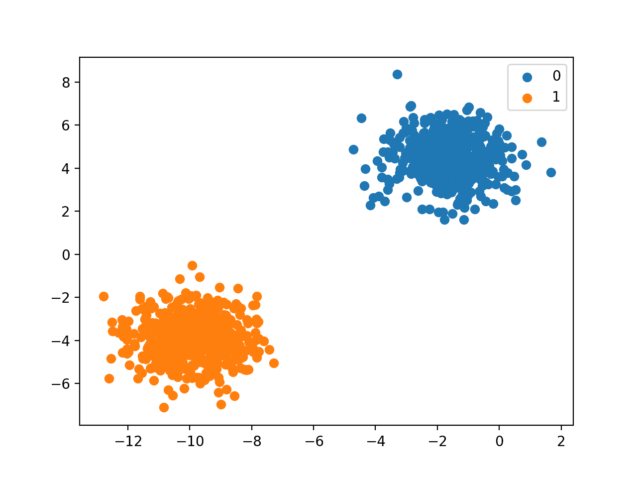
Finally, a scatter plot is created for the input variables in the dataset and the points are colored based on their class value.
We can see two distinct clusters that we might expect would be easy to discriminate.
 https://machinelearningmastery.com/wp-content/uploads/2020/01/Scatter-Plot-of-Binary-Classification-Dataset-300x225.png 300w, https://machinelearningmastery.com/wp-content/uploads/2020/01/Scatter-Plot-of-Binary-Classification-Dataset-1024x768.png 1024w, https://machinelearningmastery.com/wp-content/uploads/2020/01/Scatter-Plot-of-Binary-Classification-Dataset-768x576.png 768w" alt="Scatter Plot of Binary Classification Dataset" width="1280" height="960">
Scatter Plot of Binary Classification Dataset
Multi-Class Classification
Multi-class classification refers to those classification tasks that have more than two class labels.
Examples include:
- Face classification.
- Plant species classification.
- Optical character recognition.
Unlike binary classification, multi-class classification does not have the notion of normal and abnormal outcomes. Instead, examples are classified as belonging to one among a range of known classes.
The number of class labels may be very large on some problems. For example, a model may predict a photo as belonging to one among thousands or tens of thousands of faces in a face recognition system.
Problems that involve predicting a sequence of words, such as text translation models, may also be considered a special type of multi-class classification. Each word in the sequence of words to be predicted involves a multi-class classification where the size of the vocabulary defines the number of possible classes that may be predicted and could be tens or hundreds of thousands of words in size.
It is common to model a multi-class classification task with a model that predicts a Multinoulli probability distribution for each example.
The Multinoulli distribution is a discrete probability distribution that covers a case where an event will have a categorical outcome, e.g. K in {1, 2, 3, …, K}. For classification, this means that the model predicts the probability of an example belonging to each class label.
Many algorithms used for binary classification can be used for multi-class classification.
Popular algorithms that can be used for multi-class classification include:
- k-Nearest Neighbors.
- Decision Trees.
- Naive Bayes.
- Random Forest.
- Gradient Boosting.
Algorithms that are designed for binary classification can be adapted for use for multi-class problems.
This involves using a strategy of fitting multiple binary classification models for each class vs. all other classes (called one-vs-rest) or one model for each pair of classes (called one-vs-one).
- One-vs-Rest: Fit one binary classification model for each class vs. all other classes.
- One-vs-One: Fit one binary classification model for each pair of classes.
Binary classification algorithms that can use these strategies for multi-class classification include:
- Logistic Regression.
- Support Vector Machine.
Next, let’s take a closer look at a dataset to develop an intuition for multi-class classification problems.
We can use the make_blobs() function to generate a synthetic multi-class classification dataset.


